Linear MPC

Basics of Linear MPC Controller for Quadruped Walking Robots

This post is sourced from pympc-quadruped and translated into Korean.

Linear Model Predictive Controller

MPC

1. Dynamic Constraints

a. Approximated Angular Velocity Dynamics

The robot’s orientation is expressed as a vector of Z-Y-X Euler angles \(\Theta = [\phi, \theta, \psi]^\text{T}\), where

• \(\psi\) is the yaw,

• \(\theta\) is the pitch, and

• \(\phi\) is the roll.

These angles correspond to a sequence of rotations such that the transform from body to world coordinates can be expressed as \[ \mathbf{R} = \mathbf{R}_z(\psi)\mathbf{R}_y(\theta)\mathbf{R}_x(\phi) \]

where \(\mathbf{R}_n(\alpha)\) represents a positive rotation of \(\alpha\) about the \(n\)-axis. In details, we can write

\[ \mathbf{R}_z(\psi) = \begin{bmatrix} \cos\psi & -\sin \psi & 0 \\ \sin\psi & \cos \psi & 0 \\ 0 & 0 & 1 \end{bmatrix}, \mathbf{R}_y(\theta) = \begin{bmatrix} \cos\theta & 0 & \sin\theta \\ 0 & 1 & 0 \\ -\sin\theta & 0 & \cos\theta \end{bmatrix}, \mathbf{R}_z(\psi) = \begin{bmatrix} \cos\psi & -\sin \psi & 0 \\ \sin\psi & \cos \psi & 0 \\ 0 & 0 & 1 \end{bmatrix} \]

From [2], we have known that \(\dot{\mathbf{R}} = [\mathbf{\omega}]\mathbf{R}\), where \(\mathbf{\omega} \in \mathbb{R}^3\) is the robot’s angular velocity, \([\mathbf{\omega}] \in \mathbb{R}^{3\times3}\) is defined as the skew-symmetric matrix with respect to \(\mathbf{\omega}\), and \(\mathbf{R}\) is the rotation matrix which transforms from body to world coordinates. Then the angular velocity in world coordinates can be found with

\[ \begin{aligned} [\mathbf{\omega}] &= \dot{\mathbf{R}}\mathbf{R}^{-1} = \dot{\mathbf{R}}\mathbf{R}^\text{T} \\ &= \left( \frac{\partial R}{\partial \psi} + \frac{\partial R}{\partial \theta} + \frac{\partial R}{\partial \phi} \right)\mathbf{R}^\text{T} \\ &= \begin{bmatrix} 0 & \dot{\phi} \sin\theta - \dot{\psi} & \dot{\theta}\cos\psi + \dot{\phi}\cos\theta\sin\psi \\ -\dot{\phi} \sin\theta + \dot{\psi} & 0 & \dot{\theta}\sin\psi - \dot{\phi}\cos\psi\cos\theta \\ -\dot{\theta}\cos\psi - \dot{\phi}\cos\theta\sin\psi & -\dot{\theta}\sin\psi + \dot{\phi}\cos\psi\cos\theta & 0 \end{bmatrix} \end{aligned} \]

The above result is easy to get using the MATLAB script.

syms psi theta phi real
syms psidot thetadot phidot real

Rz = [cos(psi), -sin(psi), 0;
      sin(psi), cos(psi),  0;
      0,        0,         1];

Ry = [cos(theta),  0, sin(theta);
      0,           1, 0;
      -sin(theta), 0, cos(theta)];
  
Rx = [1, 0,        0;
      0, cos(phi), -sin(phi);
      0, sin(phi), cos(phi)];
  
R = simplify(Rz*Ry*Rx);

Somega = simplify((diff(R,phi)*phidot + diff(R,theta)*thetadot + diff(R,psi)*psidot) * R')

Now we are ready to build connections between the angular velocity in world coordinates \(\mathbf{\omega}\) and the rate of change of Euler angles \(\dot{\mathbf{\Theta}} = [\dot{\phi}, \dot{\theta}, \dot{\psi}]^\text{T}\).

\[ \mathbf{\omega} = \begin{bmatrix} -\dot{\theta}\sin\psi + \dot{\phi}\cos\psi\cos\theta \\ \dot{\theta}\cos\psi + \dot{\phi}\cos\theta\sin\psi \\ -\dot{\phi} \sin\theta + \dot{\psi} \end{bmatrix} = \begin{bmatrix} \cos\theta\cos\psi & -\sin\psi & 0 \\ \cos\theta\sin\psi & \cos\psi & 0 \\ -\sin\theta & 0 & 1 \end{bmatrix}\begin{bmatrix} \dot{\phi} \\ \dot{\theta} \\ \dot{\psi} \end{bmatrix} = \mathbf{E}\dot{\mathbf{\Theta}} \]

If the robot is not pointed vertically, which means \(\cos\theta \neq 0\), the matrix \(\mathbf{E}\) is invertable. In such case, we can get

\[ \dot{\mathbf{\Theta}} = \mathbf{E}^{-1}\mathbf{\omega} = \begin{bmatrix} \frac{\cos\psi}{\cos\theta} & \frac{\sin\psi}{\cos\theta} & 0 \\ -\sin\psi & \cos\psi & 0 \\ \cos\psi\tan\theta & \sin\psi\tan\theta & 1 \end{bmatrix}\mathbf{\omega} \]

For small values of roll \(\phi\) and pitch \(\theta\), the above equation can be approximated as

\[ \dot{\mathbf{\Theta}} \approx \begin{bmatrix} \cos\psi & \sin\psi & 0 \\ -\sin\psi & \cos\psi & 0 \\ 0 & 0 & 1 \end{bmatrix} \mathbf{\omega} \]

which is equivalent to

\[ \dot{\mathbf{\Theta}} \approx \mathbf{R}_z^\text{T} \mathbf{\omega} \tag{1} \]

Note that the order in which the Euler angle rotations are defined is important; with an alternate sequence of rotations, the approximation will be inaccurate for reasonable robot orientations.

b. Simplified Single Rigid Body Model

The predictive controller models the robot as a single rigid body subject to forces at the contact patches. Although ignoring leg dynamics is a major simplification, the controller is still able to stabilize a high-DoF system and is robust to these multi-body effects.

For the Cheetah 3 robot, this simplification is reasonable: the mass of the legs is roughly 10% of the robot's total mass

For each ground reaction force \(\mathbf{f}_i \in \mathbb{R}^3\), the vector from the CoM to the point where the force is applied is \(\mathbf{r}_i \in \mathbb{R}^3\). The rigid body dynamics in world coordinates are given by

\[ \begin{aligned} \ddot{\mathbf{p}} &= \frac{\sum_{i=1}^n\mathbf{f}_i}{m} - \mathbf{g} \\ \frac{\text{d}}{\text{d}t}(\mathbf{I\omega}) &= \sum_{i=1}^n \mathbf{r}_i \times \mathbf{f}_i\\ \dot{\mathbf{R}} &= [\mathbf{\omega}]\mathbf{R} \end{aligned} \tag{2} \]

where \(\mathbf{p} \in \mathbb{R}^3\) is the robot’s position in world frame, \(m \in \mathbb{R}\) is the robot’s mass, \(\mathbf{g} \in \mathbb{R}^3\) is the acceleration of gravity, and \(\mathbf{I} \in \mathbb{R}^3\) is the robot’s inertia tensor.

변수 정리

• \(\mathbf{f}\): 지면 반발력
• \(\mathbf{r}_i\): 질량 중심(CoM)에서 힘이 작용하는 지점까지의 벡터
• \(\mathbf{p}\): world frame에서 robot position

The nonlinear dynamics in the second and third equation of (2) motivate the approximations to avoid the nonconvex optimization that would otherwise be required for model predictive control.

(2)의 두 번째와 세 번째 방정식에서 나타나는 비선형 동역학은, 모델 예측 제어에서 요구되는 nonconvex 최적화를 피하기 위해 근사화를 도입해야 할 필요성을 제시합니다.

2번째 식

The second equation in (2) can be approximated with:

\[ \frac{\text{d}}{\text{d}t}(\mathbf{I\omega}) = \mathbf{I\dot{\omega}} + \omega \times (\mathbf{I\omega}) \approx \mathbf{I\dot{\omega}} = \sum_{i=1}^n \mathbf{r}_i \times \mathbf{f}_i \tag{3} \]

This approximation has been made in other people’s work. The \(\omega \times (\mathbf{I\omega})\) term is small for bodies with small angular velocities and does not contribute significantly to the dynamics of the robot. The inertia tensor in the world coordinate system can be found with

이 근사는 다른 연구에서도 사용되었습니다. \(\omega \times (\mathbf{I\omega})\) 항은 작은 각속도를 가지는 물체에서는 작으며, 로봇의 동역학에 크게 영향을 미치지 않습니다. 월드 좌표계에서의 inertia tensor는 다음과 같이 구할 수 있습니다.

\[ \mathbf{I} = \mathbf{R}\mathbf{I}_{\mathcal{B}}\mathbf{R}^\text{T} \]

where \(\mathbf{I}_\mathcal{B}\) is the inertia tensor in body coordinates. For small roll and pitch angles, This can be approximated by

\[ \mathbf{\hat{I}} = \mathbf{R}_z(\psi)\mathbf{I}_{\mathcal{B}}\mathbf{R}_z(\psi)^\text{T} \tag{4} \]

where \(\mathbf{\hat{I}}\) is the approximated robot’s inertia tensor in world frame. Combining equations (3)(4), we get

\[ \mathbf{\dot{\omega}} = \mathbf{\hat{I}}^{-1}\sum_{i=1}^n \mathbf{r}_i \times \mathbf{f}_i = \mathbf{\hat{I}}^{-1}\sum_{i=1}^n [\mathbf{r}_i] \mathbf{f}_i \tag{5} \]

3번째 식

For the third equation of (2), we have made the approximation in section 1.a, which gives us \[ \dot{\mathbf{\Theta}} \approx \mathbf{R}_z^\text{T} \mathbf{\omega} \]

c. Continuous-Time State Space Model

From the discussion above, we can write the simplified single rigid body model using equations (1)(2)

\[ \begin{aligned} \dot{\mathbf{\Theta}} &= \mathbf{R}_z^\text{T} \mathbf{\omega} \\ \dot{\mathbf{p}} &= \dot{\mathbf{p}} \\ \mathbf{\dot{\omega}} &= \mathbf{\hat{I}}^{-1}\sum_{i=1}^n [\mathbf{r}_i] \mathbf{f}_i \\ \ddot{\mathbf{p}} &= \frac{\sum_{i=1}^n\mathbf{f}_i}{m} - \mathbf{g} \end{aligned} \tag{6} \]

In matrix form:

\[ \begin{bmatrix} \mathbf{\dot{\Theta}} \\ \mathbf{\dot{p}} \\ \mathbf{\dot{\omega}} \\ \mathbf{\ddot{p}} \end{bmatrix} = \begin{bmatrix} \mathbf{0}_3 & \mathbf{0}_3 & \mathbf{R}_z^\text{T} & \mathbf{0}_3 \\ \mathbf{0}_3 & \mathbf{0}_3 & \mathbf{0}_3 & \mathbf{I}_3 \\ \mathbf{0}_3 & \mathbf{0}_3 & \mathbf{0}_3 & \mathbf{0}_3 \\ \mathbf{0}_3 & \mathbf{0}_3 & \mathbf{0}_3 & \mathbf{0}_3 \end{bmatrix} \begin{bmatrix} \mathbf{\Theta} \\ \mathbf{p} \\ \mathbf{\omega} \\ \mathbf{\dot{p}} \end{bmatrix} + \begin{bmatrix} \mathbf{0}_3 & \mathbf{0}_3 & \mathbf{0}_3 & \mathbf{0}_3 \\ \mathbf{0}_3 & \mathbf{0}_3 & \mathbf{0}_3 & \mathbf{0}_3 \\ \mathbf{\hat{I}}^{-1}[\mathbf{r}_1] & \mathbf{\hat{I}}^{-1}[\mathbf{r}_1] & \mathbf{\hat{I}}^{-1}[\mathbf{r}_1] & \mathbf{\hat{I}}^{-1}[\mathbf{r}_1]\\ \frac{\mathbf{I}_3}{m} & \frac{\mathbf{I}_3}{m} & \frac{\mathbf{I}_3}{m} & \frac{\mathbf{I}_3}{m} \end{bmatrix} \begin{bmatrix} \mathbf{f}_1 \\ \mathbf{f}_2 \\ \mathbf{f}_3 \\ \mathbf{f}_4 \end{bmatrix} + \begin{bmatrix} \mathbf{0}_{31} \\ \mathbf{0}_{31} \\ \mathbf{0}_{31} \\ -\mathbf{g} \end{bmatrix} \]

This equation can be rewritten with an additional gravity state \(g\) (note that here \(g\) is a scalar) to put the dynamics into the convenient state-space form: \[ \dot{\mathbf{x}}(t) = \mathbf{A_c}(\psi)\mathbf{x}(t) + \mathbf{B_c}(\mathbf{r}_1, \cdots, \mathbf{r}_4, \psi)\mathbf{u}(t) \tag{7} \]

where \(\mathbf{A_c} \in \mathbb{R}^{13\times13}\) and \(\mathbf{B_c} \in \mathbb{R}^{13\times12}\).

In details, we have \[ \begin{bmatrix} \mathbf{\dot{\Theta}} \\ \mathbf{\dot{p}} \\ \mathbf{\dot{\omega}} \\ \mathbf{\ddot{p}} \\ -\dot{g} \end{bmatrix} = \begin{bmatrix} \mathbf{0}_3 & \mathbf{0}_3 & \mathbf{R}_z^\text{T} & \mathbf{0}_3 & 0\\ \mathbf{0}_3 & \mathbf{0}_3 & \mathbf{0}_3 & \mathbf{I}_3 & 0\\ \mathbf{0}_3 & \mathbf{0}_3 & \mathbf{0}_3 & \mathbf{0}_3 & 0\\ \mathbf{0}_3 & \mathbf{0}_3 & \mathbf{0}_3 & \mathbf{0}_3 & \mathbf{e}_z\\ 0 & 0 & 0 & 0 & 0 \end{bmatrix} \begin{bmatrix} \mathbf{\Theta} \\ \mathbf{p} \\ \mathbf{\omega} \\ \mathbf{\dot{p}} \\ -g \end{bmatrix} + \begin{bmatrix} \mathbf{0}_3 & \mathbf{0}_3 & \mathbf{0}_3 & \mathbf{0}_3 \\ \mathbf{0}_3 & \mathbf{0}_3 & \mathbf{0}_3 & \mathbf{0}_3 \\ \mathbf{\hat{I}}^{-1}[\mathbf{r}_1] & \mathbf{\hat{I}}^{-1}[\mathbf{r}_1] & \mathbf{\hat{I}}^{-1}[\mathbf{r}_1] & \mathbf{\hat{I}}^{-1}[\mathbf{r}_1]\\ \frac{\mathbf{I}_3}{m} & \frac{\mathbf{I}_3}{m} & \frac{\mathbf{I}_3}{m} & \frac{\mathbf{I}_3}{m} \\ 0 & 0 & 0 & 0 \end{bmatrix} \begin{bmatrix} \mathbf{f}_1 \\ \mathbf{f}_2 \\ \mathbf{f}_3 \\ \mathbf{f}_4 \end{bmatrix} \tag{8} \]

This form depends only on yaw and footstep locations. If these can be computed ahead of time, the dynamics become linear time-varying, which is suitable for convex model predictive control.

이 형태는 오직 yaw와 발걸음 위치에만 의존합니다. 만약 이것들이 미리 계산될 수 있다면, 동역학은 선형 시간 변화 형태가 되어 convex model predictive control에 적합해집니다.

d. Discretization

See https://en.wikipedia.org/wiki/Discretization for more details about the purposed method.

\[ \exp\left(\begin{bmatrix} \mathbf{A_c} & \mathbf{B_c} \\ \mathbf{0} & \mathbf{0} \end{bmatrix} \text{dt}\right) = \begin{bmatrix} \mathbf{A_d} & \mathbf{B_d} \\ \mathbf{0} & \mathbf{I} \end{bmatrix} \tag{9} \]

This allows us to express the dynamics in the discrete time form

\[ \mathbf{x}[k+1] = \mathbf{A_d} \mathbf{x}[k] + \mathbf{B_d}[k]\mathbf{u}[k] \tag{10} \]

The above approximation is only accurate if the robot is able to follow the reference trajectory. Large deviations from the reference trajectory, possibly caused by external or terrain disturbances, will result in \(\mathbf{B_d}[k]\) being inaccurate. However, for the first time step, \(\mathbf{B_d}[k]\) is calculated from the current robot state, and will always be correct. If, at any point, the robot is disturbed from following the reference trajectory, the next iteration of the MPC, which happens at most 40 ms after the disturbance, will recompute the reference trajectory based on the disturbed robot state, allowing it compensate for a disturbance.

위 근사는 로봇이 reference trajectory을 따라갈 수 있을 때만 정확합니다. 외부 요인이나 지형의 방해로 인해 reference trajectory에서 크게 벗어나는 경우, \(\mathbf{B_d}[k]\)가 부정확해질 수 있습니다.

그러나 first timestep에서는 \(\mathbf{B_d}[k]\)가 현재 로봇 상태에서 계산되므로 항상 정확합니다. 어떤 시점에서든 로봇이 참조 궤적에서 벗어나 방해를 받는다면, 방해가 발생한 후 최대 40ms 이내에 실행되는 MPC의 다음 반복에서, 방해를 받은 로봇 상태를 기반으로 reference trajectory을 재계산하여 방해를 보정할 수 있습니다.

2. Force Constraints

a. Equality Constraints(등식조건)

The equality constraint

\[ \mathbf{D}_k \mathbf{u}_k = \mathbf{0} \tag{11} \]

is used to set all forces from feet off the ground to zero, enforcing the desired gait, where \(\mathbf{D}_k\) is a matrix which selects forces corresponding with feet not in contact with the ground at timestep \(k\).

지면에서 떨어진 발들에 작용하는 모든 힘을 0으로 설정하여 원하는 gait을 강제하기 위해 사용됩니다. 여기서 \(\mathbf{D}_k\)는 시간 단계 \(k\)에서 지면에 접촉하지 않은 발들에 해당하는 힘을 선택하는 행렬입니다.

b. Inequality Constraints(부등식조건)

The inequality constraints limit the minimum and maximum \(z\)-force as well as a square pyramid approximation of the friction cone.

부등식 제약 조건은 최소 및 최대 \(z\)-힘을 제한하며, friction cone의 사각뿔 근사를 포함합니다.

For each foot, we have the following 10 inequality constraints (\(i = 1,2,3,4\)).

\[ \begin{aligned} f_{\min} \leq &f_{i,z} \leq f_{\max} \\ -\mu f_{i,z} \leq &f_{i,x} \leq \mu f_{i,z} \\ -\mu f_{i,z} \leq &f_{i,y} \leq \mu f_{i,z} \end{aligned} \]

We want to write these constraints in matrix form. Thus we need to look these equations in detail.

For example, the constraints \(-\mu f_{i,z} \leq \pm f_{i,x} \leq \mu f_{i,z}\) actually are \[ \begin{aligned} -\mu f_{i,z} &\leq f_{i,x} \\ -\mu f_{i,z} &\leq -f_{i,x} \\ f_{i,x} &\leq \mu f_{i,z} \\ -f_{i,x} &\leq \mu f_{i,z} \end{aligned} \]

We can rewrite these equations as

\[ \begin{aligned} f_{i,x} + \mu f_{i,z} &\geq 0 \\ -f_{i,x} + \mu f_{i,z} &\geq 0 \\ f_{i,x} - \mu f_{i,z} &\leq 0 \\ -f_{i,x} - \mu f_{i,z} &\leq 0 \end{aligned} \]

We can see that the first two equations and the last two equations are the same. Thus we can use the first two equations to replace these four equations. We can also note that \(f_{\min} = 0\) as always. With the observation discussed above, we can write the force constraints for one foot on the ground as

\[ \begin{bmatrix} 0 \\ 0 \\ 0 \\ 0 \\ 0 \end{bmatrix} \leq \begin{bmatrix} 1 & 0 & \mu \\ -1 & 0 & \mu \\ 0 & 1 & \mu \\ 0 & -1 & \mu \\ 0 & 0 & 1 \end{bmatrix} \begin{bmatrix} f_{i,x} \\ f_{i,y} \\ f_{i,z} \end{bmatrix} \leq \begin{bmatrix} \infty \\ \infty \\ \infty \\ \infty \\ f_{\max} \end{bmatrix} \]

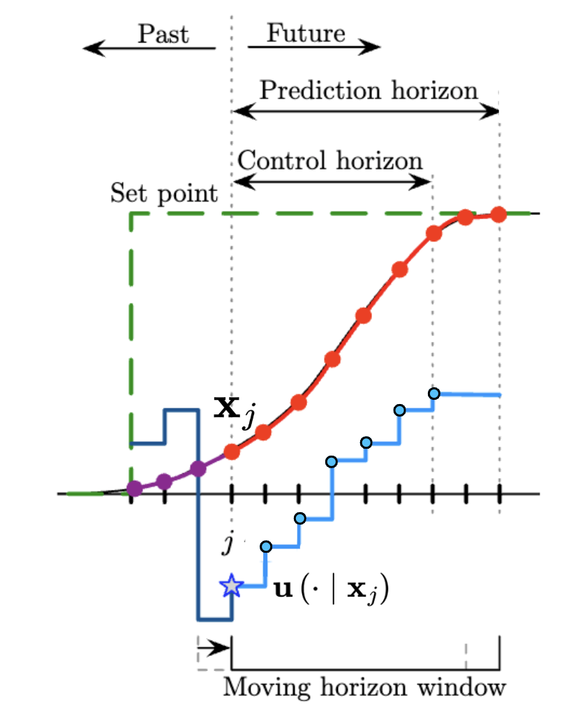
3. Reference Trajectory Generation

The desired robot behavior is used to construct the reference trajectory. In the application, our reference trajectories are simple and only contain non-zero \(xy\)-velocity, \(xy\)-position, \(z\)-postion, yaw, and yaw rate. All parameters are commanded directly by the robot operator except for yaw and \(xy\)-position, which are determined by integrating the appropriate velocities. The other states (roll, pitch, roll rate, pitch rate and \(z\)-velocity) are always set to 0. The reference trajectory is also used to determine the dynamics constraints and future foot placement locations.

In practice, the reference trajectory is short (between 0.5 and 0.3 seconds) and recalculated often (every 0.05 to 0.03 seconds) to ensure the simplified dynamics remain accurate if the robot is disturbed.

4. QP Formulation

a. Batch Formulation for Dynamic Constraints

Key idea: For the state space model, express \(x_0, x_1, \cdots, x_k\) as function of \(u_0\).

\[ \begin{aligned} x_1 &= Ax_0 + Bu_0 \\ x_2 &= Ax_1 + Bu_1 = A^2x_0 + ABu_0 + Bu_1 \\ &\vdots \\ x_k & = A^kx_0 + A^{k-1}Bu_0 + A^{k-2}Bu_1 + \cdots + Bu_{k-1} \end{aligned} \]

We can write these equations in matrix form

\[ \begin{bmatrix} x_1 \\ x_2 \\ \vdots \\ x_k \end{bmatrix} = \begin{bmatrix} A \\ A^2 \\ \vdots \\A^k \end{bmatrix} x_0 + \begin{bmatrix} B & 0 & \cdots & 0 \\ AB & B & \cdots & 0 \\ \vdots & \vdots & \ddots & \vdots \\ A^{k-1}B & A^{k-2}B & \cdots & B \end{bmatrix} \begin{bmatrix} u_0 \\ u_1 \\ \vdots \\ u_{k-1} \end{bmatrix} \]

where \(k\) is the horizon length. Let \(x_t\) denotes the system state at time step \(t\), i.e. at current state, then we can write

\[ \begin{bmatrix} x_{t+1} \\ x_{t+2} \\ \vdots \\ x_{t+k} \end{bmatrix} = \begin{bmatrix} A \\ A^2 \\ \vdots \\A^k \end{bmatrix} x_t + \begin{bmatrix} B & 0 & \cdots & 0 \\ AB & B & \cdots & 0 \\ \vdots & \vdots & \ddots & \vdots \\ A^{k-1}B & A^{k-2}B & \cdots & B \end{bmatrix} \begin{bmatrix} u_t \\ u_{t+1} \\ \vdots \\ u_{t+k-1} \end{bmatrix} \]

We can denote this equation as

\[ X = S^x x_t + S^u U \]

For a 2-norm cost function, we can write

\[ \begin{aligned} J_k(x_t,\mathbf{U}) &= J_f(x_k) + \sum_{i=0}^{k-1}l(x_i,u_i) \\ &= x_k^\text{T} Q_f x_k + \sum_{i=0}^{k-1}\left(x_i^\text{T}Q_ix_i + u_i^\text{T}R_iu_i\right) \\ &= X^\text{T}\bar{Q}X + U^\text{T}\bar{R}U \end{aligned} \]

where

\[ \mathbf{U} = \begin{bmatrix} X \\ U \end{bmatrix} \quad \bar{Q} = \begin{bmatrix} Q_1 & & & \\ & \ddots & & \\ & & Q_{k-1} & \\ & & & Q_f \end{bmatrix} \quad \bar{R} = \begin{bmatrix} R & & \\ & \ddots & \\ & & R \\ \end{bmatrix} \]

Substituting the expression of state space model into the cost, we have

\[ \begin{aligned} J_k(x_t,\mathbf{U}) &= X^\text{T}\bar{Q}X + U^\text{T}\bar{R}U \\ &= \left(S^x x_t + S^u U\right)^\text{T}\bar{Q}\left(S^x x_t + S^u U\right) + U^\text{T}\bar{R}U \\ &= U^\text{T}\underbrace{\left((S^u)^\text{T}\bar{Q}S^u+\bar{R}\right)}_H U + 2x_t^\text{T}\underbrace{(S^x)^\text{T}\bar{Q}S^u}_F U + x_t^\text{T}\underbrace{(S^x)^\text{T}\bar{Q}S^x}_Y x_t\\ &= U^\text{T}HU + 2x_tFU + x_t^\text{T}Yx_t \end{aligned} \] Compare with the standard form of cost in QP formulation \(\frac{1}{2}U^\text{T}HU + U^\text{T}g\), we can easily get \[ \begin{aligned} H &= 2\left((S^u)^\text{T}\bar{Q}S^u + \bar{R}\right) \\ g &= 2(S^u)^\text{T}\bar{Q}S^xx_t \end{aligned} \]

b. Create QP Cost

Recall that the form of our MPC problem is

\[ \begin{aligned} \min_{x, u} \quad& \sum_{i=0}^{k-1}(x_{i+1}-x_{i+1,\text{ref}})^{\text{T}}Q_i(x_{i+1}-x_{i+1,\text{ref}}) + u_i^\text{T}R_iu_i \\ \text{s.t.} \quad& x_{i+1} = A_ix_i + B_iu_i \\ & \underline{c}_i \leq C_iu_i \leq \overline{c}_i \\ & D_iu_i = 0 \end{aligned} \]

where \(i = 0, \cdots, k-1\).

In this project, we choose \(Q_1 = \cdots = Q_{k-1} = Q_f\), i.e.

\[ \bar{Q} = \begin{bmatrix} Q & & & \\ & \ddots & & \\ & & Q & \\ & & & Q \end{bmatrix} \quad \bar{R} = \begin{bmatrix} R & & \\ & \ddots & \\ & & R \\ \end{bmatrix} \]

_Qi = np.diag(np.array(parameters['Q'], dtype=float))
Qbar = np.kron(np.identity(horizon), _Qi)

_r = parameters['R']
_Ri = _r * np.identity(num_input, dtype=float)
Rbar = np.kron(np.identity(horizon), _Ri)

Let’s substitute the dynamic constraint into the cost function, then we can get

\[ \begin{aligned} J &= \sum_{i=0}^{k-1}(x_{i+1}-x_{i+1,\text{ref}})^{\text{T}}Q_i(x_{i+1}-x_{i+1,\text{ref}}) + u_i^\text{T}R_iu_i \\ &= \sum_{i=0}^{k-1}(A_ix_i+B_iu_i-x_{i+1,\text{ref}})^{\text{T}}Q_i(A_ix_i + B_iu_i-x_{i+1,\text{ref}}) + u_i^\text{T}R_iu_i \\ &= (S^x x_t + S^u U - X_{\text{ref}})^\text{T}\bar{Q}(S^x x_t + S^u U - X_\text{ref}) + U^\text{T}\bar{R}U \end{aligned} \]

where \(X_\text{ref} = [x_{1,\text{ref}}, \cdots, x_{k,\text{ref}}]^\text{T}\). We can get the QP matrix with the same procedure.

\[ \begin{aligned} H &= 2\left((S^u)^\text{T}\bar{Q}S^u + \bar{R}\right) \\ g &= 2(S^u)^\text{T}\bar{Q}(S^xx_t-X_\text{ref}) \end{aligned} \]

c. Create QP Constraint

d. QP Solver

qpsolvers: https://pypi.org/project/qpsolvers/

As mentioned in the project description of qpsolvers, we need to write our formulation in the form

\[ \begin{aligned} \min_x &\quad \frac{1}{2}x^\text{T}Px + q^\text{T}x \\ \text{s.t.} & \quad Gx \leq h \\ &\quad Ax = b \\ &\quad \text{lb} \leq x \leq \text{ub} \end{aligned} \]

Then we can get the solution using the code below

from qpsolvers import solve_qp
x = solve_qp(P, q, G, h, A, b, lb, ub)
print("QP solution: x = {}".format(x))

The QP problem in the paper is written as

\[ \begin{aligned} \min_\mathbf{U} &\quad \frac{1}{2}\mathbf{U}^\text{T}\mathbf{HU} + \mathbf{U}^\text{T}\mathbf{g} \\ \text{s.t.} &\quad \underline{\mathbf{c}} \leq \mathbf{CU} \leq \overline{\mathbf{c}} \end{aligned} \]

Reference

[1] Di Carlo J., Wensing P. M., Katz B., et al. Dynamic Locomotion in the MIT Cheetah 3 Through Convex Model-Predictive Control[C]//2018 IEEE/RSJ International Conference on Intelligent Robots and Systems (IROS). IEEE, 2018: 1-9. [PDF]

[2] Bledt G, Powell M J, Katz B, et al. Mit cheetah 3: Design and Control of a Robust, Dynamic Quadruped Robot[C]//2018 IEEE/RSJ International Conference on Intelligent Robots and Systems (IROS). IEEE, 2018: 2245-2252. [PDF]